A train travelling at 20 m s1 starts to accelerate with constant acceleration. It covers the next kilometre in 25 seconds. Use the equation s = ut+at2 to calculate the acceleration. Find also how fast the train is moving at the end of this time. Illustrate the motion of the train with a velocity-time graph. How long does the train take to cover the first half kilometre?

Spread the love

3 October 2023 by alevelmechanics1.com

Title: Journey Unleashed: Acceleration Chronicles of a Train

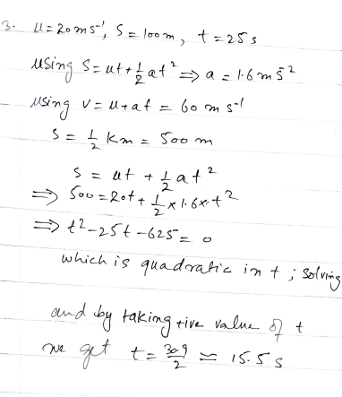
Introduction: In the rhythmic cadence of its journey, a train initially cruising at 20 m/s decides to embark on an acceleration odyssey. This numerical exploration navigates through the acceleration chronicles, uncovering the train’s acceleration and its velocity at a specific juncture. The interplay of distance, time, and acceleration comes to life through the lens of the equation s = ut + at², offering insights into the train’s dynamic journey.

Scenario Overview: Picture the train, a behemoth of motion, accelerating with a constant force, gracefully covering the next kilometer in 25 seconds. This voyage of acceleration propels the train into realms of dynamic velocity.

Objectives: The primary objectives include deciphering the train’s acceleration through the application of the kinematic equation and determining its velocity at the conclusion of the acceleration phase. Additionally, the exploration unveils the temporal nuances of the train’s journey, particularly the time taken to traverse the first half kilometer.

Significance: Understanding the acceleration dynamics and the resultant velocity is pivotal in grasping the train’s ability to transform its initial speed into a newfound momentum. Furthermore, the temporal markers add layers to the narrative of the train’s journey.

Acceleration Chronicles: The numerical exploration unfolds the mathematical tapestry of the train’s acceleration, employing the equation s = ut + at² to demystify the force shaping its trajectory. The calculated acceleration becomes a key parameter in comprehending the train’s dynamic journey.

Mathematical Calculations: Leveraging the kinematic equation, the acceleration is calculated, and the subsequent determination of the velocity at the end of the acceleration phase adds depth to the analysis. The temporal dimensions, especially the time taken to cover the first half kilometer, are unraveled through mathematical precision.

Visualization: A visual symphony in the form of a velocity-time graph encapsulates the train’s acceleration chronicles, tracing the evolution of velocity with temporal progression.

Douglas Quadling Mechanics 1
Exercise 1B Q3

Conclusion:

As the train unfurls its acceleration chronicles, this numerical exploration deciphers the intricacies of its journey. The calculated acceleration becomes a testament to the force propelling the train, and the velocity at a specific juncture offers a snapshot of its dynamic momentum. The velocity-time graph visually encapsulates the rhythmic dance between speed and time. In unraveling the temporal markers, the exploration sheds light on the train’s ability to traverse distances with calculated precision, showcasing the dynamic essence of its accelerated journey

CategoriesChapter 1, Exercise 1B

A marathon competitor running at 5 m s1 puts on a sprint when she is 100 metres from the finish, and covers this distance in 16 seconds. Assuming that her acceleration is constant, use the equation s= = (u+v)t to find how fast she is running as she crosses the finishing line.

A long-jumper takes a run of 30 metres to accelerate to a speed of 10 m s1 from a standing start. Find the time he takes to reach this speed, and hence calculate his acceleration. Illustrate his run-up with a velocity-time graph.

Logged in as alevelmechanics1.com. Edit your profile. Log out? Required fields are marked *