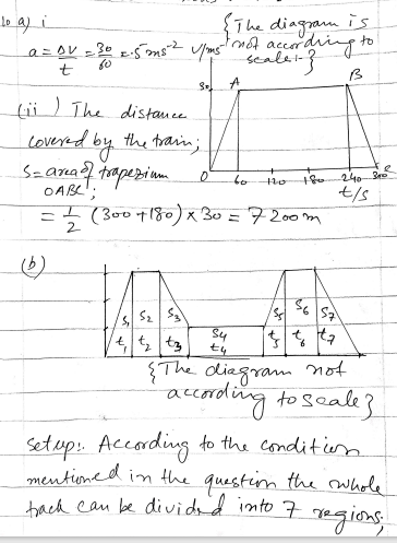
A train travels from a station P to the next station Q, arriving at Q exactly 5 minutes after leaving P…………..
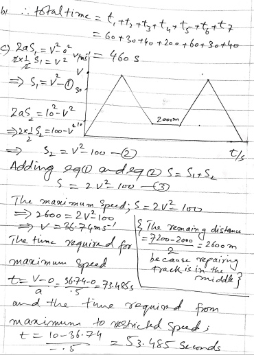
(b)On one occasion, when the track is being repaired, the train is restricted to a maximum speed of 10 ms for the 2000 m length of track lying midway between P and Q.. The train always accelerates and decelerates at the rate shown in the figure. When not accelerating or decelerating or moving at the restricted speed of 10 m s1, the train travels at 30 ms1. Sketch the (t,v) graph for the train’s journey from P to Q when the speed restriction is in force, and hence find how long the train takes to travel from P to on this occasion.
(c)The second figure shows the (t,v) graph for the train accelerating from rest up to a maximum speed of V ms and then immediately decelerating to a speed of 10 ms. The acceleration and deceleration have the same value as shown in the first figure. Show that the distance travelled is (2V2-100) metres.
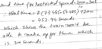
Determine whether the train in (b) could, by exceeding the normal speed of 30 m s when possible, make up the time lost due to the speed restriction when travelling from P to Q. Assume that the acceleration and deceleration must remain as before.
Title: Dynamics of Train Journey: Acceleration, Distance, and Time
1. Introduction:
A train travels from a station P to the next station Q, arriving at Q exactly 5 minutes after leaving P….
- The scenario unfolds as a train embarks on a journey from station P to the next station Q, characterized by a (t,v) graph with three straight line segments approximating its acceleration and velocity profile.
2. Scenario Description:
- The journey comprises accelerations, decelerations, and speed restrictions, demanding an analysis of the train’s dynamics to answer critical questions about acceleration, distance, and time.
3. Objectives:
- (i) Calculate the acceleration of the train during the first minute.
- (ii) Determine the distance from P to Q.
4. Significance:
- Understanding the intricacies of the train’s (t,v) graph sheds light on the dynamic nature of its journey, addressing real-world challenges such as speed restrictions and optimizing travel time.
5. Exploration Focus:
- The exploration delves into the nuances of acceleration and speed restrictions, culminating in a comprehensive understanding of the train’s journey.
6. Dynamics of Acceleration:
- (i) Calculation of the train’s acceleration during the first minute sets the stage for unraveling the initial phase of its journey.
7. Distance Computation:
- (ii) Determining the distance from P to Q involves integrating the velocity-time graph, providing insights into the spatial aspects of the train’s travel.
8. Speed Restriction Scenario:
- The scenario introduces a speed restriction, prompting the sketching of an altered (t,v) graph and exploration of the time taken to travel from P to Q under these conditions.
9. Acceleration and Deceleration Profile:
- (c) Analyzing the (t,v) graph for acceleration and deceleration from rest to a maximum speed and then decelerating to 10 m/s, unveiling the distance traveled as (2V² – 100) meters.
10. Time Optimization Challenge:
- Evaluating whether the train, by exceeding its normal speed of 30 m/s, can compensate for time lost due to speed restrictions, with assumptions about constant acceleration and deceleration.
11. Practical Implications:
- Findings contribute to the practical understanding of optimizing train journeys, addressing challenges posed by speed restrictions and seeking time efficiency
Douglas Quadling Mechanics1 Miscellaneous Exercise1 Q10(a)& Q10(b)
A train travels from a station P to the next station Q, arriving at Q exactly 5 minutes after leaving P……

Douglas Quadling Mechanics1 Miscellaneous Exercise1 Q10(b)&Q10(c)
A train travels from a station P to the next station Q, arriving at Q exactly 5 minutes after leaving P…….


Scope: Dynamics of Train Journey
1. Introduction:
A train travels from a station P to the next station Q, arriving at Q exactly 5 minutes after leaving P……
- The scope of this numerical revolves around a train’s journey from station P to Q, characterized by a (t,v) graph with three straight line segments. The primary objective is to delve into the dynamics of the train’s acceleration, distances covered, and time considerations.
2. Scenario Analysis:
- The exploration encompasses scenarios where the train experiences accelerations, decelerations, and speed restrictions. The goal is to unravel the intricacies of the train’s journey, providing insights into real-world challenges and optimizing travel dynamics.
3. Objectives:
- (i) Calculate the acceleration of the train during the first minute of its journey.
- (ii) Determine the distance from P to Q, utilizing the velocity-time graph.
4. Significance:
- The significance lies in understanding the nuances of the train’s (t,v) graph, addressing critical questions about acceleration, distance covered, and the impact of speed restrictions on the overall journey.
5. Dynamics of Acceleration:
- A specific focus is given to the calculation of the train’s acceleration during the initial minute, providing a foundational understanding of the acceleration profile.
6. Distance Computation:
- The exploration involves integrating the velocity-time graph to compute the distance from P to Q. This spatial analysis contributes to the overall comprehension of the train’s travel.
7. Speed Restriction Scenario:
- An additional layer of complexity is introduced with a speed restriction scenario. The scope extends to sketching an altered (t,v) graph and determining the time taken for the train to travel from P to Q under these conditions.
8. Acceleration and Deceleration Profile:
- A separate analysis considers the (t,v) graph depicting acceleration from rest to a maximum speed and then decelerating to 10 m/s. The objective is to show that the distance traveled is (2V² – 100) meters.
9. Time Optimization Challenge:
- The scope extends to exploring whether the train, by exceeding its normal speed of 30 m/s, can compensate for time lost due to speed restrictions. Assumptions include constant acceleration and deceleration.
10. Practical Implications:
- Findings from this exploration hold practical implications for optimizing train journeys, addressing challenges posed by speed restrictions, and seeking efficient time management in transit.
Conclusion:
A train travels from a station P to the next station Q, arriving at Q exactly 5 minutes after leaving P……
- The overall scope promises to unveil the dynamic facets of the train’s journey, providing a comprehensive perspective on acceleration, distances covered, and time considerations during its voyage from P to Q.
The Next Question: https://alevelmechanics1.com/614/if-a-ball-is-placed-on-a-straight-sloping-track-and-then-released/
