A long-jumper takes a run of 30 metres to accelerate to a speed of 10 m s1 from a standing start. Find the time he takes to reach this speed, and hence calculate his acceleration. Illustrate his run-up with a velocity-time graph.

3 October 2023 by alevelmechanics1.com

Title: Leap into Motion: Long-Jumper’s Acceleration Adventure

---

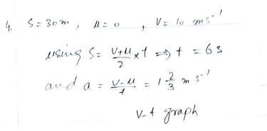
Introduction: Embarking on the runway of anticipation, a long-jumper, poised for a remarkable leap, undertakes a run-up to accelerate from a standstill to a speed of 10 m/s. This numerical exploration seeks to unravel the temporal intricacies of the acceleration journey, calculating the time it takes for the long-jumper to attain the desired speed. Additionally, the acceleration experienced during this acceleration adventure will be unveiled. The long-jumper’s run-up is encapsulated through the lens of a velocity-time graph.

Scenario Overview: Imagine the long-jumper, ready to defy gravity, initiating a run-up that spans a distance of 30 meters. This runway serves as the canvas for acceleration, propelling the athlete to a speed of 10 m/s.

Objective: The primary objective is to calculate the time it takes for the long-jumper to accelerate from a standstill to the target speed of 10 m/s. Subsequently, the calculated time is employed to unveil the acceleration experienced during this acceleration journey. The velocity-time graph visually encapsulates the dynamic interplay between velocity and time.

Significance: Understanding the temporal and acceleration dynamics of the run-up is pivotal in comprehending the athlete’s performance. It provides insights into the time required to achieve the desired speed and the intensity of acceleration during this athletic endeavor.

Acceleration Adventure: The numerical exploration delves into the temporal dimensions of the long-jumper’s run-up, unfolding the sequence of events from the standing start to the exhilarating speed of 10 m/s. The calculated time becomes a temporal marker of the acceleration adventure.

Mathematical Calculations: Leveraging kinematic equations, the time required for the long-jumper to attain the target speed is unveiled. The subsequent calculation divulges the acceleration experienced by the athlete, quantifying the intensity of the acceleration adventure.

Visualization: A visual representation in the form of a velocity-time graph brings the acceleration adventure to life, capturing the dynamic evolution of velocity during the run-up.

Douglas Quadling Mechanics 1
Exercise 1B Q4

Conclusion:

As the long-jumper surges through the run-up, this numerical exploration unravels the temporal intricacies of acceleration. The calculated time signifies the duration of the acceleration journey, and the derived acceleration value quantifies the athlete’s prowess in converting the runway’s expanse into velocity. The long-jumper’s acceleration adventure, a prelude to the leap, finds numerical expression in the interplay of distance, time, and acceleration.

CategoriesChapter 1, Exercise 1B

A train travelling at 20 m s1 starts to accelerate with constant acceleration. It covers the next kilometre in 25 seconds. Use the equation s = ut+at2 to calculate the acceleration. Find also how fast the train is moving at the end of this time. Illustrate the motion of the train with a velocity-time graph. How long does the train take to cover the first half kilometre?

Starting from rest, an aircraft accelerates to its take-off speed of 60 m s1 in a distance of 900 metres. Assuming constant acceleration, find how long the take-off run lasts. Hence calculate the acceleration.

Leave a comment

Logged in as alevelmechanics1.com. Edit your profile. Log out? Required fields are marked *